Distributions#

Distributions are used in the Dead Leaves Model to sample object parameters such as size, aspect ratio, orientation, color, and texture. They are specified as dictionaries with the distribution type as key and its parameters as values.

Constant#

The Constant distribution returns a fixed deterministic value every time it is sampled. Use this when you want a parameter to remain unchanged.

Use case: Fixed parameter for all leaves.

{
    "constant": {
        "value": <value>
    }
}

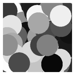
Example: Constant size

../_images/8dfb4baecbf7b3011f02a5dc80c3350317d4a4e8d298223d6c8721eaf1385a5c.png

Uniform (from PyTorch)#

The Uniform distribution samples values evenly from a range [low, high] (where \(a=\)low and \(b=\)high).

\[\begin{split} f(x) = \begin{cases} \frac{1}{b-a}, & \text{for } x\in[a,b] \\ 0, &\text{else}.\end{cases} \end{split}\]

Use case: Random but equally likely values, e.g. random orientation or hue.

{
    "uniform": {
        "low": <value>, 
        "high": <value>
    }
}

Example: Uniform size and luminance

../_images/8a35ce5717b8ba44c72f089aae295ff1f10ac6bb7d30f5c39fcdbf08fb581548.png

Normal (from PyTorch)#

The Normal distribution samples values from a Gaussian (bell-shaped) distribution with mean \(\mu=\)loc and standard deviation \(\sigma=\)scale.

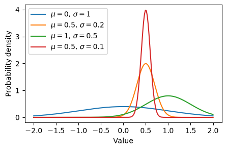
\[ f(x) = \frac{1}{\sigma\sqrt{2\pi}}\exp\left(-\frac{1}{2}\left(\frac{x-\mu}{\sigma}\right)^2\right) \]

../_images/151bda41a8e0d4a1304d6fe758c6e060e3c1e2d964e6e8e10c543cfa11faebc3.png

Use case: Gaussian noise or color.

{
    "normal": {
        "loc": <value>, 
        "scale": <value>
    }
}

Example: Normal size and luminance

../_images/720f40c86051a8f4016d241cf0d564b4144a3439b4074663692991019a285a69.png

Beta (from PyTorch)#

The Beta distribution samples values in the range [0,1] and is controlled by two concentration parameters \(\alpha=\)concentration0 and \(\beta=\)concentration1.

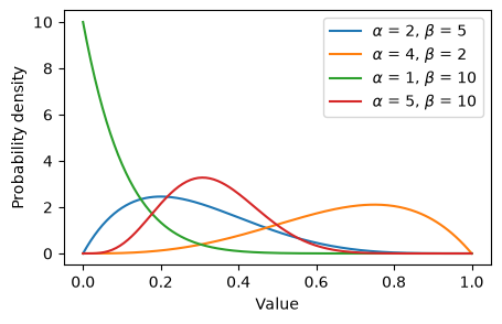
\[\begin{split} f(x) = \begin{cases} \frac{x^{\alpha-1}(1-x)^{\beta-1}}{B(\alpha,\beta)}, &\text{for } x\in[0,1] \\ 0, &\text{else.} \end{cases} \end{split}\]

../_images/6ea7bb27ff545b413a05553d03f40a0a788dc9c66ef8e6c43d90629774aeba82.png

Use case: Random proportions or normalized parameters, e.g. aspect ratio or blending factors.

{
    "beta": {
        "concentration0": <value>, 
        "concentration1": <value>
    }
}

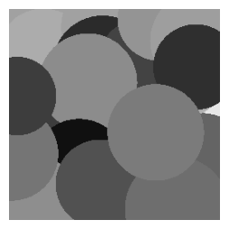
Example: Beta aspect ratio

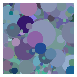
../_images/f0dbb0357d9d85c2fde70232e260b56c486732fab97bc3f5e20784e78bce4007.png

Poisson (from PyTorch)#

The Poisson distribution generates integer counts based on a given rate \(\lambda\).

\[ P(k) = e^{-\lambda}\frac{\lambda^k}{k!} \]

../_images/fa2726c4668a20d51cef79ea80133d68a8013e21cddb865306a14b6fc380be67.png

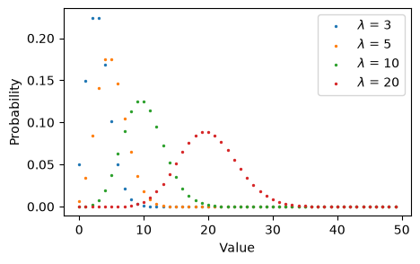
Use case: Polygons with random number of vertices.

{
    "poisson": {
        "rate": <value>
    }
}

Example: Polygons with Poisson vertices number

---------------------------------------------------------------------------
ValueError                                Traceback (most recent call last)
Cell In[8], line 11
       "n_vertices": {"poisson": {"rate": 5}},
       },
   (256,256)
)
---> 11 leaf_table, segmentation_map = model.generate_segmentation()

colormodel = LeafAppearanceSampler(leaf_table)
colormodel.sample_color({"gray": {"uniform": {"low": 0.0, "high": 1.0}}})

File ~/checkouts/readthedocs.org/user_builds/deadleaves/checkouts/latest/deadleaves/deadleaves.py:335, in LeafGeometryGenerator.generate_segmentation(self)
   continue
# Compute AABB, clip to canvas, query live tiles
--> 335 y_min, x_min, y_max, x_max = leaf_mask_kw[self.leaf_shape].bbox(
   params
)  # pyright: ignore[reportCallIssue]
y_min = max(y_min, 0)
x_min = max(x_min, 0)

File ~/checkouts/readthedocs.org/user_builds/deadleaves/checkouts/latest/deadleaves/leaf_masks.py:304, in leaf_aabb(params, leaf_shape)
   area = float(params["area"])
   n_v = int(params["n_vertices"])
--> 304     r = math.sqrt(2 * area / (n_v * math.sin(2 * math.pi / n_v)))
   return (
       math.floor(cy - r),
       math.floor(cx - r),
       math.ceil(cy + r),
       math.ceil(cx + r),
   )
# Fallback — unknown shape, return infinite box (no acceleration)

ValueError: math domain error

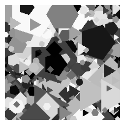
Powerlaw#

The PowerLaw distribution is useful for heavy-tailed sizes, common in natural phenomena. It is parameterized via a lower (low, \(x_\min\)) and an upper bound (high, \(x_\max\)) and the exponent \(k\).

\[\begin{split} f(x) = \begin{cases} \frac{k-1}{x_{\min}^{1-k}-x_{\max}^{1-k}}\cdot x^{-k}, & \text{for } x\in[x_{\min}, x_{\max}] \\ 0, & \text{else.} \end{cases} \end{split}\]

For continuity with respect to \(k\) the distribution for \(k=1\) is given by

\[\begin{split} f(x) = \begin{cases} \frac{1}{\ln(x_{\max})-\ln(x_{\min})}\cdot x^{-1}, & \text{for } x\in[x_{\min}, x_{\max}] \\ 0, & \text{else.} \end{cases} \end{split}\]

For \(k=0\) the distribution equals a uniform distribution between the lower and the upper bound.

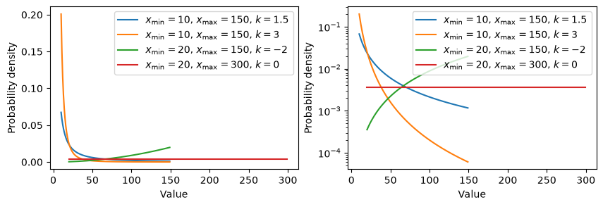
Use case: Generating leaf sizes with many small and few large objects.

{
    "powerlaw": {
        "low": <value>, 
        "high": <value>, 
        "k": <value>
    }
}

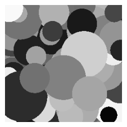
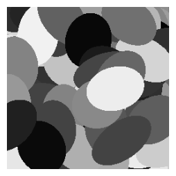
Example: Powerlaw size and saturation

Cosine#

The Cosine distribution produces periodic variations for values between \(-\pi\) and \(\pi\):

\[\begin{split} f(x) = \begin{cases} \frac{1}{2\pi} \left(1+A\cdot\cos(F\cdot x)\right), & \text{for } x\in[-\pi,\pi] \\ 0, & \text{else.} \end{cases} \end{split}\]

The frequency, \(F\) has to be an integer and specifies the number of phases on the value range. The amplitude, \(A\) changes the intensity between 0.0 and 1.0.

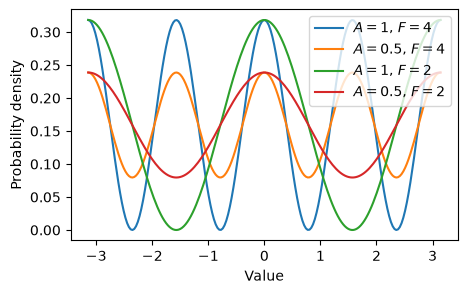
Use case: Orientations of phase-like variations with periodic structure.

{
    "cosine": {
        "amplitude": <value>, 
        "frequency": <value>
    }
}

Note

Random variables with this distribution always produce values between \(-\pi\) and \(\pi\) and are mainly useful to parameterized orientation distributions.

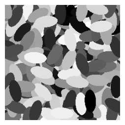
Example: Cosine orientation

Expcosine#

The ExpCosine distribution is a sharply peaked periodic distribution, useful for strongly directional parameters.

\[\begin{split} f(x) = \begin{cases} \frac{\exp\left(-c \cdot \sqrt{1 - \cos(F \cdot x)}\right)}{\int_{-\pi}^{\pi} f(x) dx}, & \text{for } x\in[-\pi,\pi] \\ 0, & \text{else.} \end{cases} \end{split}\]

The frequency, \(F\) has to be an integer and specifies the number of periodic peaks on the value range. The positive exponential_constant, \(c\) sets the strength of the peak.

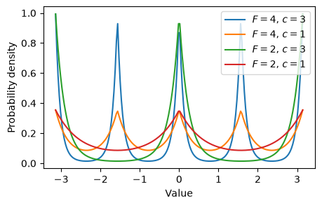
Use case: Leaf orientations with a strong preferred direction, e.g. cardinal bias.

{
    "expcosine": {
        "frequency": <value>,
        "exponential_constant": <value>
    }
}

Note

Random variables with this distribution always produce values between \(-\pi\) and \(\pi\) and are mainly useful to parameterized orientation distributions.

Example: Exponential cosine orientation

Image#

The Image distribution samples from a set of image files in a given directory. The class will discover all image type files in dir and uniformly sample images from the list.

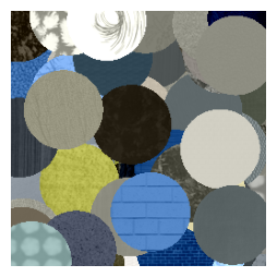
Use case: Assign color or texture by sampling existing images or texture patches, respectively.

{
    "image": {
        "dir": <value>
    }
}

Note

Sampling from this distribution will return one or multiple paths to image(s) in dir. In particular, it will sample from all available image files in the directory provided.

Example: Color and texture from images